3.2 Data structures
Now that you’ve been introduced to some of the most important classes of data in R, let’s have a look at some of main structures that we have for storing these data.
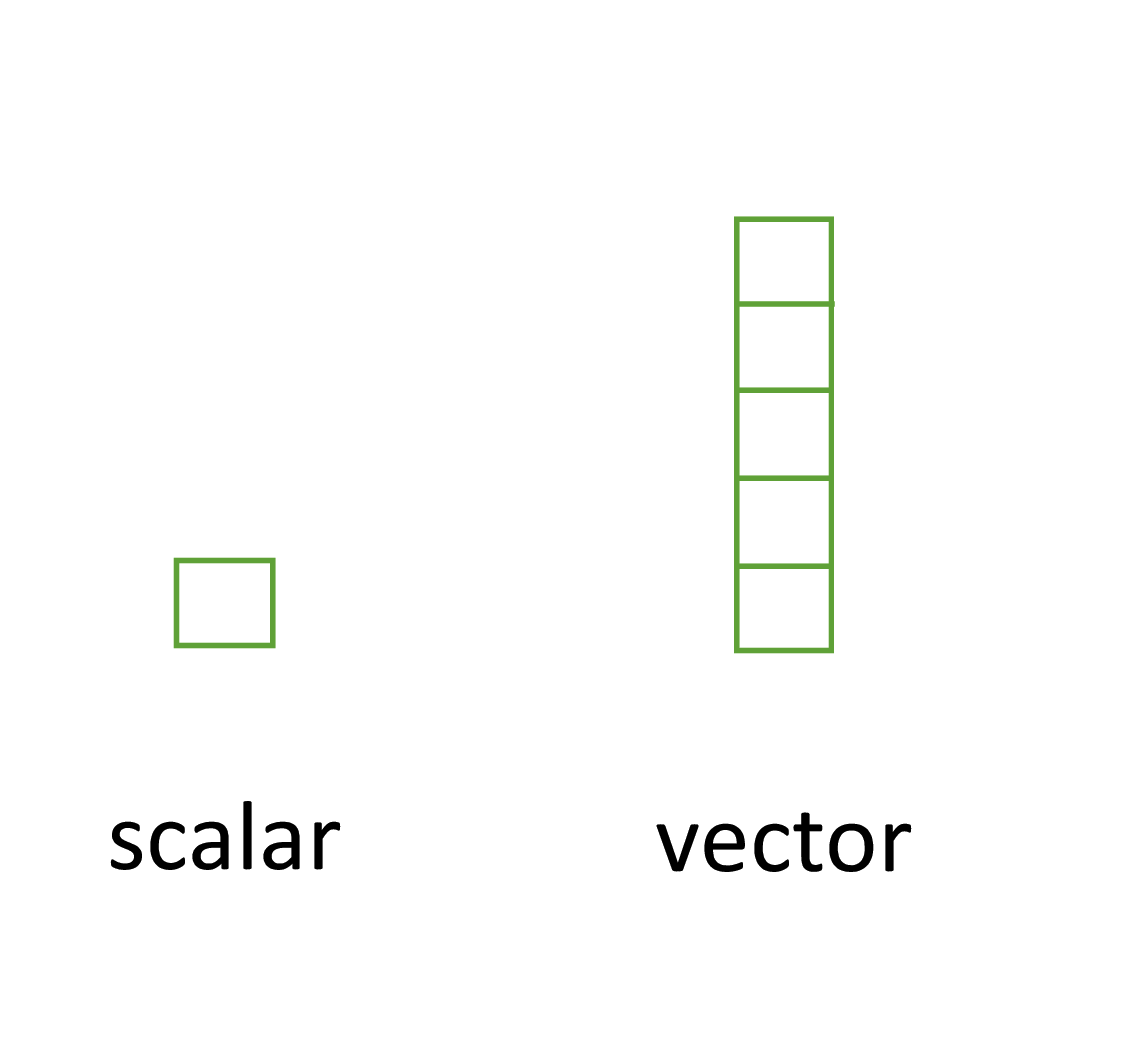
3.2.1 Scalars and vectors
Perhaps the simplest type of data structure is the vector. You’ve already been introduced to vectors in Chapter 2 although some of the vectors you created only contained a single value. Vectors that have a single value (length 1) are called scalars. Vectors can contain numbers, characters, factors or logicals, but the key thing to remember is that all the elements inside a vector must be of the same class. In other words, vectors can contain either numbers, characters or logicals but not mixtures of these types of data. There is one important exception to this, you can include NA (remember this is special type of logical) to denote missing data in vectors with other data types.
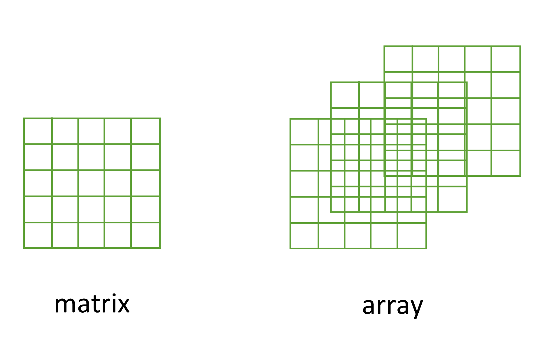
3.2.2 Matrices and arrays
Another useful data structure used in many disciplines such as population ecology, theoretical and applied statistics is the matrix. A matrix is simply a vector that has additional attributes called dimensions. Arrays are just multidimensional matrices. Again, matrices and arrays must contain elements all of the same data class.
A convenient way to create a matrix or an array is to use the matrix() and array() functions respectively. Below, we will create a matrix from a sequence 1 to 16 in four rows (nrow = 4) and fill the matrix row-wise (byrow = TRUE) rather than the default column-wise. When using the array() function we define the dimensions using the dim = argument, in our case 2 rows, 4 columns in 2 different matrices.
my_mat <- matrix(1:16, nrow = 4, byrow = TRUE)
my_mat
##      [,1] [,2] [,3] [,4]
## [1,]    1    2    3    4
## [2,]    5    6    7    8
## [3,]    9   10   11   12
## [4,]   13   14   15   16

my_array <- array(1:16, dim = c(2, 4, 2))
my_array
## , , 1
##
##      [,1] [,2] [,3] [,4]
## [1,]    1    3    5    7
## [2,]    2    4    6    8
##
## , , 2
##
##      [,1] [,2] [,3] [,4]
## [1,]    9   11   13   15
## [2,]   10   12   14   16
Sometimes it’s also useful to define row and column names for your matrix but this is not a requirement. To do this use the rownames() and colnames() functions.
rownames(my_mat) <- c("A", "B", "C", "D")
colnames(my_mat) <- c("a", "b", "c", "d")
my_mat
##    a  b  c  d
## A  1  2  3  4
## B  5  6  7  8
## C  9 10 11 12
## D 13 14 15 16
Once you’ve created your matrices you can do useful stuff with them and as you’d expect, R has numerous built in functions to perform matrix operations. Some of the most common are given below. For example, to transpose a matrix we use the transposition function t().
my_mat_t <- t(my_mat)
my_mat_t
##   A B  C  D
## a 1 5  9 13
## b 2 6 10 14
## c 3 7 11 15
## d 4 8 12 16
To extract the diagonal elements of a matrix and store them as a vector we can use the diag() function.
The usual matrix addition, multiplication etc can be performed. Note the use of the %*% operator to perform matrix multiplication.
mat.1 <- matrix(c(2, 0, 1, 1), nrow = 2)    # notice that the matrix has been filled
mat.1                                     # column-wise by default
##      [,1] [,2]
## [1,]    2    1
## [2,]    0    1

mat.2 <- matrix(c(1, 1, 0, 2), nrow = 2)
mat.2
##      [,1] [,2]
## [1,]    1    0
## [2,]    1    2

mat.1 + mat.2           # matrix addition
##      [,1] [,2]
## [1,]    3    1
## [2,]    1    3
mat.1 * mat.2           # element by element products
##      [,1] [,2]
## [1,]    2    0
## [2,]    0    2
mat.1 %*% mat.2         # matrix multiplication
##      [,1] [,2]
## [1,]    3    2
## [2,]    1    2
3.2.3 Lists
The next data structure we will quickly take a look at is a list. Whilst vectors and matrices are constrained to contain data of the same type, lists are able to store mixtures of data types. In fact we can even store other data structures such as vectors and arrays within a list or even have a list of a list. This makes for a very flexible data structure which is ideal for storing irregular or non-rectangular data (see Chapter 7 for an example).
To create a list we can use the list() function. Note how each of the three list elements are of different classes (character, logical, and numeric) and are of different lengths.
list_1 <- list(c("black", "yellow", "orange"),
               c(TRUE, TRUE, FALSE, TRUE, FALSE, FALSE),
               matrix(1:6, nrow = 3))
list_1
## [[1]]
## [1] "black"  "yellow" "orange"
##
## [[2]]
## [1]  TRUE  TRUE FALSE  TRUE FALSE FALSE
##
## [[3]]
##      [,1] [,2]
## [1,]    1    4
## [2,]    2    5
## [3,]    3    6
Elements of the list can be named during the construction of the list
list_2 <- list(colours = c("black", "yellow", "orange"),
               evaluation = c(TRUE, TRUE, FALSE, TRUE, FALSE, FALSE),
               time = matrix(1:6, nrow = 3))
list_2
## $colours
## [1] "black"  "yellow" "orange"
##
## $evaluation
## [1]  TRUE  TRUE FALSE  TRUE FALSE FALSE
##
## $time
##      [,1] [,2]
## [1,]    1    4
## [2,]    2    5
## [3,]    3    6
or after the list has been created using the names() function.
3.2.4 Data frames
Take a look at this video for a quick introduction to data frame objects in R
By far the most commonly used data structure to store data in is the data frame. A data frame is a powerful two-dimensional object made up of rows and columns which looks superficially very similar to a matrix. However, whilst matrices are restricted to containing data all of the same type, data frames can contain a mixture of different types of data. Typically, in a data frame each row corresponds to an individual observation and each column corresponds to a different measured or recorded variable. This setup may be familiar to those of you who use LibreOffice Calc or Microsoft Excel to manage and store your data. Perhaps a useful way to think about data frames is that they are essentially made up of a bunch of vectors (columns) with each vector containing its own data type but the data type can be different between vectors.
As an example, the data frame below contains the results of an experiment to determine the effect of removing the tip of petunia plants (Petunia sp.) grown at 3 levels of nitrogen on various measures of growth (note: data shown below are a subset of the full dataset). The data frame has 8 variables (columns) and each row represents an individual plant. The variables treat and nitrogen are factors (categorical variables). The treat variable has 2 levels (tip and notip) and the nitrogen level variable has 3 levels (low, medium and high). The variables height, weight, leafarea and shootarea are numeric and the variable flowers is an integer representing the number of flowers. Although the variable block has numeric values, these do not really have any order and could also be treated as a factor (i.e. they could also have been called A and B).
| treat | nitrogen | block | height | weight | leafarea | shootarea | flowers |
|---|---|---|---|---|---|---|---|
| tip | medium | 1 | 7.5 | 7.62 | 11.7 | 31.9 | 1 |
| tip | medium | 1 | 10.7 | 12.14 | 14.1 | 46.0 | 10 |
| tip | medium | 1 | 11.2 | 12.76 | 7.1 | 66.7 | 10 |
| tip | medium | 1 | 10.4 | 8.78 | 11.9 | 20.3 | 1 |
| tip | medium | 1 | 10.4 | 13.58 | 14.5 | 26.9 | 4 |
| tip | medium | 1 | 9.8 | 10.08 | 12.2 | 72.7 | 9 |
| notip | low | 2 | 3.7 | 8.10 | 10.5 | 60.5 | 6 |
| notip | low | 2 | 3.2 | 7.45 | 14.1 | 38.1 | 4 |
| notip | low | 2 | 3.9 | 9.19 | 12.4 | 52.6 | 9 |
| notip | low | 2 | 3.3 | 8.92 | 11.6 | 55.2 | 6 |
| notip | low | 2 | 5.5 | 8.44 | 13.5 | 77.6 | 9 |
| notip | low | 2 | 4.4 | 10.60 | 16.2 | 63.3 | 6 |
There are a couple of important things to bear in mind about data frames. These types of objects are known as rectangular data (or tidy data) as each column must have the same number of observations. Also, any missing data should be recorded as an NA just as we did with our vectors.
We can construct a data frame from existing data objects such as vectors using the data.frame() function. As an example, let’s create three vectors p.height, p.weight and p.names and include all of these vectors in a data frame object called dataf.
p.height <- c(180, 155, 160, 167, 181)
p.weight <- c(65, 50, 52, 58, 70)
p.names <- c("Joanna", "Charlotte", "Helen", "Karen", "Amy")

dataf <- data.frame(height = p.height, weight = p.weight, names = p.names)
dataf
##   height weight     names
## 1    180     65    Joanna
## 2    155     50 Charlotte
## 3    160     52     Helen
## 4    167     58     Karen
## 5    181     70       Amy
You’ll notice that each of the columns are named with variable name we supplied when we used the data.frame() function. It also looks like the first column of the data frame is a series of numbers from one to five. Actually, this is not really a column but the name of each row. We can check this out by getting R to return the dimensions of the dataf object using the dim() function. We see that there are 5 rows and 3 columns.
Another really useful function which we use all the time is str() which will return a compact summary of the structure of the data frame object (or any object for that matter).
str(dataf)
## 'data.frame':    5 obs. of  3 variables:
##  $ height: num  180 155 160 167 181
##  $ weight: num  65 50 52 58 70
##  $ names : chr  "Joanna" "Charlotte" "Helen" "Karen" ...
The str() function gives us the data frame dimensions and also reminds us that dataf is a data.frame type object. It also lists all of the variables (columns) contained in the data frame, tells us what type of data the variables contain and prints out the first five values. We often copy this summary and place it in our R scripts with comments at the beginning of each line so we can easily refer back to it whilst writing our code. We showed you how to comment blocks in RStudio here.
Also notice that R has automatically decided that our p.names variable should be a character (chr) class variable when we first created the data frame. Whether this is a good idea or not will depend on how you want to use this variable in later analysis. If we decide that this wasn’t such a good idea we can change the default behaviour of the data.frame() function by including the argument stringsAsFactors = TRUE. Now our strings are automatically converted to factors.
p.height <- c(180, 155, 160, 167, 181)
p.weight <- c(65, 50, 52, 58, 70)
p.names <- c("Joanna", "Charlotte", "Helen", "Karen", "Amy")

dataf <- data.frame(height = p.height, weight = p.weight, names = p.names,
                                        stringsAsFactors = TRUE)
str(dataf)
## 'data.frame':    5 obs. of  3 variables:
##  $ height: num  180 155 160 167 181
##  $ weight: num  65 50 52 58 70
##  $ names : Factor w/ 5 levels "Amy","Charlotte",..: 4 2 3 5 1