3.6 Exporting data
By now we hope you’re getting a feel for how powerful and useful R is for manipulating and summarising data (and we’ve only really scratched the surface). One of the great benefits of doing all your data wrangling in R is that you have a permanent record of all the things you’ve done to your data. Gone are the days of making undocumented changes in Excel or Calc! By treating your data as ‘read only’ and documenting all of your decisions in R you will have made great strides towards making your analysis more reproducible and transparent to others. It’s important to realise, however, that any changes you’ve made to your data frame in R will not change the original data file you imported into R (and that’s a good thing). Happily it’s straightforward to export data frames to external files in a wide variety of formats.
3.6.1 Export functions
The main workhorse function for exporting data frames is the write.table() function. As with the read.table() function, the write.table() function is very flexible with lots of arguments to help customise it’s behaviour. As an example, let’s take our original flowers data frame, do some useful stuff to it and then export these changes to an external file.
Let’s order the rows in the data frame in ascending order of height within each level nitrogen. We will also apply a square root transformation on the number of flowers variable (flowers) and a log10 transformation on the height variable and save these as additional columns in our data frame (hopefully this will be somewhat familiar to you!).
flowers_df2 <- flowers[order(flowers$nitrogen, flowers$height), ]
flowers_df2$flowers_sqrt <- sqrt(flowers_df2$flowers)
flowers_df2$log10_height <- log10(flowers_df2$height)
str(flowers_df2)
## 'data.frame':    96 obs. of  10 variables:
##  $ treat       : chr  "notip" "notip" "notip" "notip" ...
##  $ nitrogen    : Factor w/ 3 levels "low","medium",..: 1 1 1 1 1 1 1 1 1 1 ...
##  $ block       : int  1 1 1 2 1 2 2 2 1 2 ...
##  $ height      : num  1.8 2.2 2.3 2.4 3 3.1 3.2 3.3 3.7 3.7 ...
##  $ weight      : num  6.01 9.97 7.28 9.1 9.93 8.74 7.45 8.92 7.03 8.1 ...
##  $ leafarea    : num  17.6 9.6 13.8 14.5 12 16.1 14.1 11.6 7.9 10.5 ...
##  $ shootarea   : num  46.2 63.1 32.8 78.7 56.6 39.1 38.1 55.2 36.7 60.5 ...
##  $ flowers     : int  4 2 6 8 6 3 4 6 5 6 ...
##  $ flowers_sqrt: num  2 1.41 2.45 2.83 2.45 ...
##  $ log10_height: num  0.255 0.342 0.362 0.38 0.477 ...
Now we can export our new data frame flowers_df2 using the write.table() function. The first argument is the data frame you want to export (flowers_df2 in our example). We then give the filename (with file extension) and the file path in either single or double quotes using the file = argument. In this example we’re exporting the data frame to a file called flowers_04_12.txt in the data directory. The col.names = TRUE argument indicates that the variable names should be written in the first row of the file and the row.names = FALSE argument stops R from including the row names in the first column of the file. Finally, the sep = "\t" argument indicates that a Tab should be used as the delimiter in the exported file.
write.table(flowers_df2, file = 'data/flowers_04_12.txt', col.names = TRUE,
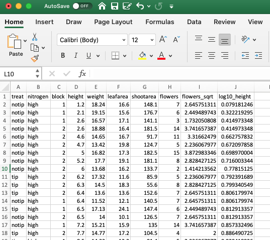
row.names = FALSE, sep = "\t")As we saved the file as a tab delimited text file we could open this file in any text editor. Perhaps a more familiar option would be to open the file in Excel. First start Excel and then select File -> Open .. in the main menu and then select our flowers_04_12.txt file to open. Next. choose the ‘Tab’ option to set the delimiter and then click on the ‘Finish’ button.
We can of course export our files in a variety of other formats. Another popular option is to export files in csv (comma separated values) format. We can do this using the write.table() function by setting the separator argument to sep = ",".
write.table(flowers_df2, file = 'data/flowers_04_12.csv', col.names = TRUE,
             row.names = FALSE, sep = ",")
Or alternatively by using the convenience function write.csv(). Notice that we don’t need to set the sep = "," or col.names = TRUE arguments as these are the defaults when using the read.csv() function.
3.6.2 Other export functions
As with importing data files into R, there are also many alternative functions for exporting data to external files beyond the write.table() function. If you followed the ‘Other import functions’ section of this Chapter you will already have the required packages installed.
The fwrite() function from the data.table package is very efficient at exporting large data objects and is much faster than the write.table() function. It’s also quite simple to use as it has most of the same arguments as write.table(). To export a tab delimited text file we just need to specify the data frame name, the output file name and file path and the separator between columns.
To export a csv delimited file it’s even easier as we don’t even need to include the sep = argument.
The readr package also comes with two useful functions for quickly writing data to external files: the write_tsv() function for writing tab delimited files and the write_csv() function for saving comma separated values (csv) files.
library(readr)
write_tsv(flowers_df2, file = 'data/flowers_04_12.txt')

write_csv(flowers_df2, file = 'data/flowers_04_12.csv')
You can even save data directly to an Excel spreadsheet using the write_excel_csv() function but again we don’t recommend this!