4.4 Multiple graphs

There are a number of different methods for plotting multiple graphs within the same graphics device, some of which you’ve already met such as pairs(), coplot(), xyplot() etc. However these functions rely on plotting multiple graphs in different panels within the same plot. If you want to plot separate plots within the same graphics device you’ll need a different approach. One of the most common methods is to use the main graphical function par() to split the plotting device up into a number of defined sections using the mfrow = argument. With this method, you first need to specify the number of rows and columns of plots you would like and then run the code for each plot. For example, to plot two graphs side by side we would use par(mfrow = c(1, 2)) to split the device into 1 row and two columns.

par(mfrow = c(1, 2))
plot(flowers$weight, flowers$shootarea, xlab = "weight",
      ylab = "shoot area")
boxplot(shootarea ~ nitrogen, data = flowers, cex.axis = 0.6)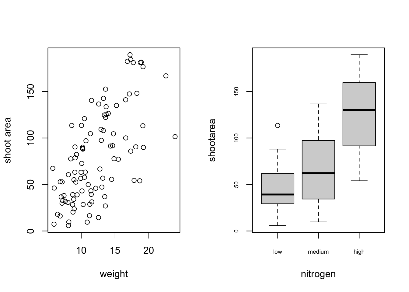

Or if we wanted to plot four plots we can split our plotting device into 2 rows and 2 columns.

par(mfrow = c(2, 2))
plot(flowers$weight, flowers$shootarea, xlab = "weight",
      ylab = "shoot area")
boxplot(shootarea ~ nitrogen, cex.axis = 0.8, data = flowers)
hist(flowers$weight, main ="")
dotchart(flowers$weight)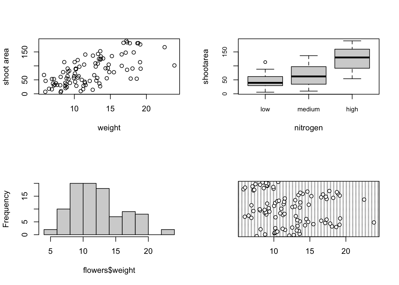

Once you’ve finished making your plots don’t forget to reset your plotting device back to normal with par(mfrow = c(1, 1)).

A more flexible approach is to use the layout() function. The layout() function allows you to split your plotting device up into different sized regions and can be used to build complex figures. Before using the layout() function we first need to specify how we’re going to split our plotting device by creating a matrix using the matrix() function (see Chapter 2 to remind yourself). Let’s create a 2 x 2 matrix.

layout_mat <- matrix(c(2, 0, 1, 3), nrow = 2, ncol = 2,
                      byrow = TRUE)
layout_mat

##      [,1] [,2]
## [1,]    2    0
## [2,]    1    3

The matrix above represents splitting the plotting device into 2 rows and 2 columns. The first plot will occupy the lower left panel, the second plot the upper left panels and the third plot the lower right panel. The upper right panel will not contain a plot as we have placed a zero here.

We can now use the layout() function to define our layout. As we have two rows and two columns we need to specify the height of each row and the width of each column using the heights = and widths = arguments. The respect = TRUE argument ensures that the units used to define the widths are the same as those to define the heights. We can get a graphical representation of our layout by using the layout.show() function.

my_lay <- layout(mat = layout_mat, 
                 heights = c(1, 3),
                 widths = c(3, 1), respect =TRUE)
layout.show(my_lay)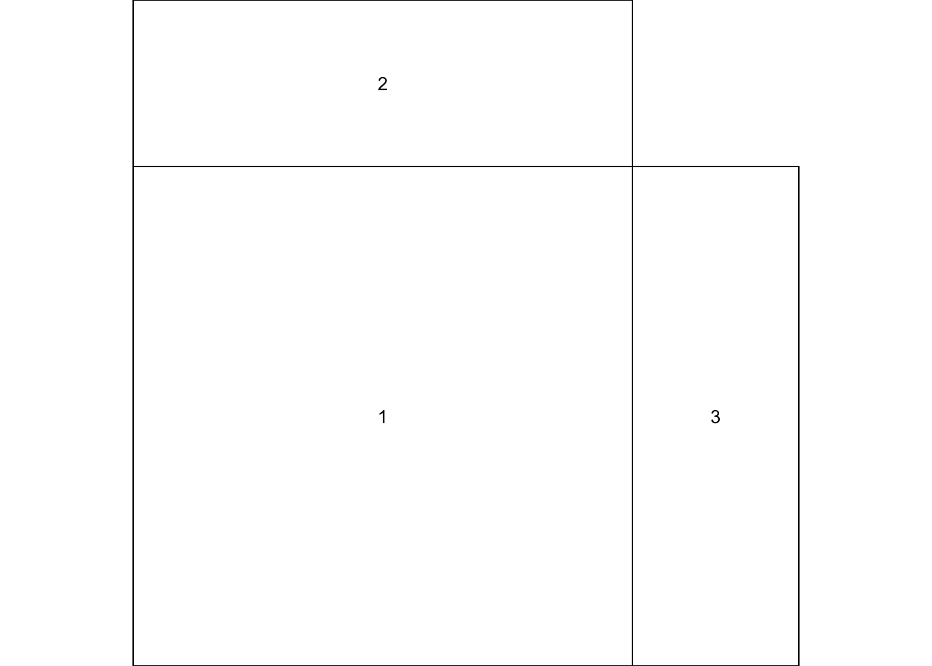

All we need to do now is create our three plots. However, before we do this we also need to change the figure margins for each of the figures using the par(mar = ) command so all of the plots can fit together in the same plotting device. This will probably take a little bit of experimenting to get the plot looking exactly how you want. For our first figure (bottom left) we will reduce the size of the bottom and left margins a little and remove the margins completely from the top and right sides with par(mar = c(4, 4, 0, 0)). For our top plot we will remove the margins from the bottom, top and right sides and set the left side to have the same margin as our first figure (par(mar = c(0, 4, 0, 0))). For the third plot on the right we will set the bottom side to have the same margin as the first plot so they line up and remove the margins from the other sides with par(mar = c(4, 0, 0, 0)).

par(mar = c(4, 4, 0, 0))
plot(flowers$weight, flowers$shootarea, 
     xlab = "weight (g)", ylab = "shoot area (cm2)")
par(mar = c(0, 4, 0, 0))
boxplot(flowers$weight, horizontal = TRUE, frame = FALSE,
        axes =FALSE)
par(mar = c(4, 0, 0, 0))
boxplot(flowers$shootarea, frame = FALSE, axes = FALSE)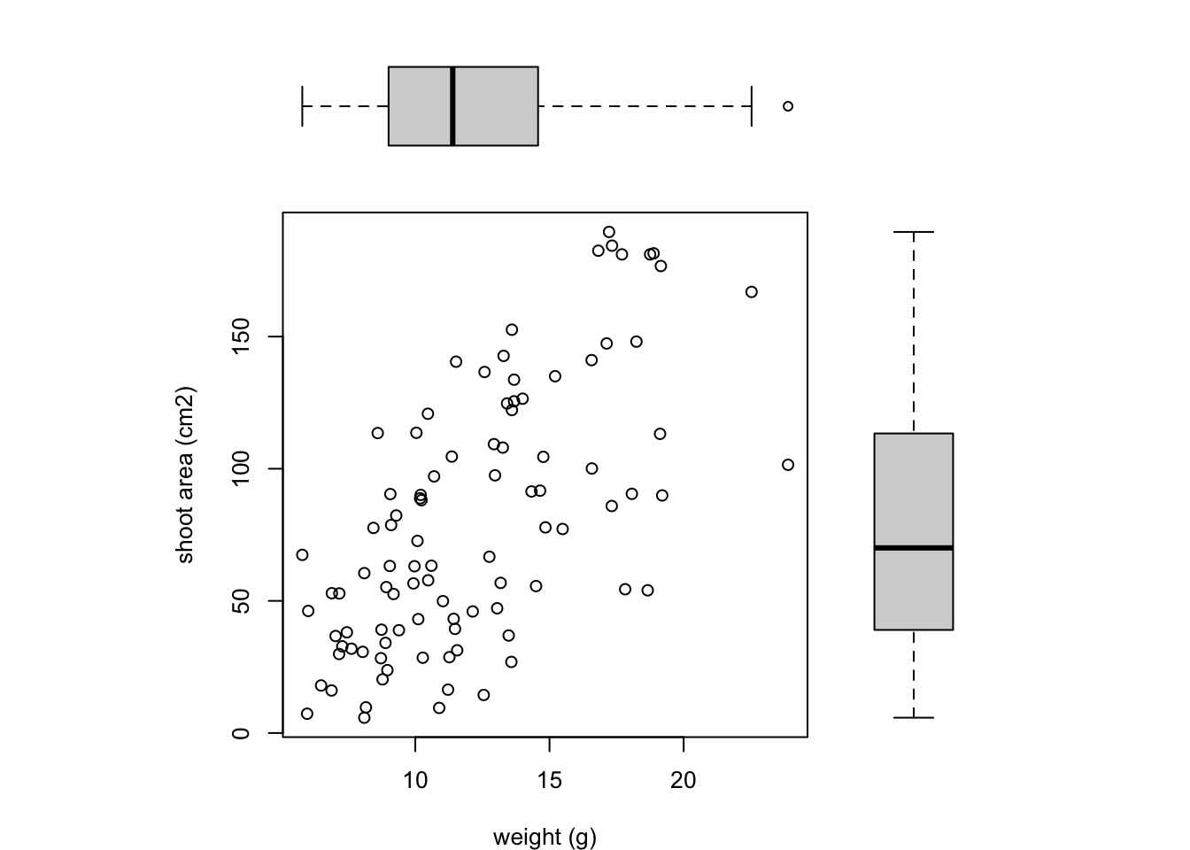

Notice we’ve specified that the boxplot at the top should be plotted horizontally with the horizontal = TRUE argument. The frame = FALSE argument prevents a border being plotted around each boxplot and the axes = FALSE argument suppresses the axes and axes labels from being plotted.