6.1 One and two sample tests
The two main functions for these types of tests are the t.test() and wilcox.test() that perform t tests and Wilcoxon’s signed rank test respectively. Both of these tests can be applied to one and two sample analyses as well as paired data.
As an example of a one sample t test we will use the trees dataset which is included with R. To access this in-built dataset we can use the data() function. This data set provides measurements of the diameter, height and volume of timber in 31 felled black cherry trees (see ?trees for more detail).
data(trees)
str(trees)
## 'data.frame':    31 obs. of  3 variables:
##  $ Girth : num  8.3 8.6 8.8 10.5 10.7 10.8 11 11 11.1 11.2 ...
##  $ Height: num  70 65 63 72 81 83 66 75 80 75 ...
##  $ Volume: num  10.3 10.3 10.2 16.4 18.8 19.7 15.6 18.2 22.6 19.9 ...
summary(trees)
##      Girth           Height       Volume
##  Min.   : 8.30   Min.   :63   Min.   :10.20
##  1st Qu.:11.05   1st Qu.:72   1st Qu.:19.40
##  Median :12.90   Median :76   Median :24.20
##  Mean   :13.25   Mean   :76   Mean   :30.17
##  3rd Qu.:15.25   3rd Qu.:80   3rd Qu.:37.30
##  Max.   :20.60   Max.   :87   Max.   :77.00
If we wanted to test whether the mean height of black cherry trees in this sample is equal to 70 ft (mu = 70), assuming these data are normally distributed, we can use a t.test() to do so.
t.test(trees$Height, mu = 70)
##
##  One Sample t-test
##
## data:  trees$Height
## t = 5.2429, df = 30, p-value = 1.173e-05
## alternative hypothesis: true mean is not equal to 70
## 95 percent confidence interval:
##  73.6628 78.3372
## sample estimates:
## mean of x
##        76
The above summary has a fairly logical layout and includes the name of the test that we have asked for (One Sample t-test), which data has been used (data: trees$Height), the t statistic, degrees of freedom and associated p value (t = 5.2, df = 30, p-value = 1e-05). It also states the alternative hypothesis (alternative hypothesis: true mean is not equal to 70) which tells us this is a two sided test (as we have both equal and not equal to), the 95% confidence interval for the mean (95 percent confidence interval:73.66 78.34) and also an estimate of the mean (sample estimates: mean of x : 76). In the above example, the p value is very small and therefore we would reject the null hypothesis and conclude that the mean height of our sample of black cherry trees is not equal to 70 ft.
The function t.test() also has a number of additional arguments which can be used for one-sample tests. You can specify that a one sided test is required by using either alternative = "greater" or alternative = "less arguments which tests whether the sample mean is greater or less than the mean specified. For example, to test whether our sample mean is greater than 70 ft.
t.test(trees$Height, mu = 70, alternative = "greater")
##
##  One Sample t-test
##
## data:  trees$Height
## t = 5.2429, df = 30, p-value = 5.866e-06
## alternative hypothesis: true mean is greater than 70
## 95 percent confidence interval:
##  74.05764      Inf
## sample estimates:
## mean of x
##        76
You can also change the confidence level used for estimating the confidence intervals using the argument conf.level = 0.99. If specified in this way, 99% confidence intervals would be estimated.
Although t tests are fairly robust against small departures from normality you may wish to use a rank based method such as the Wilcoxon’s signed rank test. In R, this is done in almost exactly the same way as the t test but using the wilcox.test() function.
wilcox.test(trees$Height, mu = 70)
## Warning in wilcox.test.default(trees$Height, mu = 70): cannot compute exact p-value with ties
## Warning in wilcox.test.default(trees$Height, mu = 70): cannot compute exact p-value with zeroes
##
##  Wilcoxon signed rank test with continuity correction
##
## data:  trees$Height
## V = 419.5, p-value = 0.0001229
## alternative hypothesis: true location is not equal to 70
Don’t worry too much about the warning message, R is just letting you know that your sample contained a number of values which were the same and therefore it was not possible to calculate an exact p value. This is only really a problem with small sample sizes. You can also use the arguments alternative = "greater" and alternative = "less".
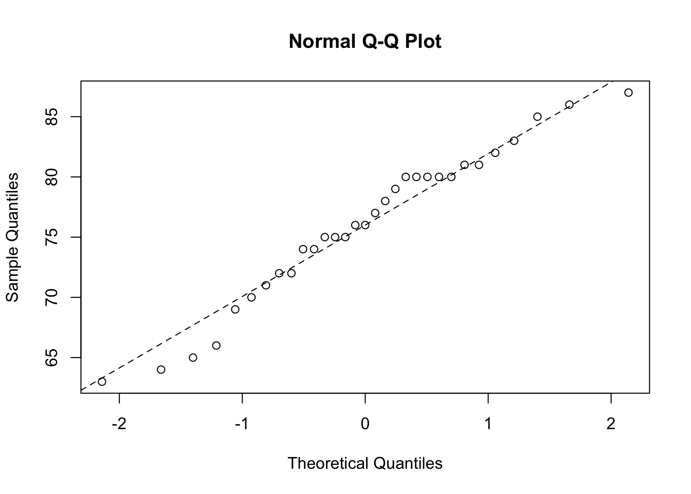
In our one sample test it’s always a good idea to examine your data for departures from normality, rather than just assuming everything is OK. Perhaps the simplest way to assess normality is the ‘quantile-quantile plot’. This graph plots the ranked sample quantiles from your distribution against a similar number of ranked quantiles taken from a normal distribution. If your data are normally distributed then the plot of your data points will be in a straight line. Departures from normality will show up as a curve or s-shape in your data points. Judging just how much departure is acceptable comes with a little bit of practice.
To construct a Q-Q plot you need to use both the qqnorm() and qqline() functions. The lty = 2 argument changes the line to a dashed line.
If you insist on performing a specific test for normality you can use the function shapiro.test() which performs a Shapiro – Wilks test of normality.
shapiro.test(trees$Height)
##
##  Shapiro-Wilk normality test
##
## data:  trees$Height
## W = 0.96545, p-value = 0.4034
In the example above, the p value = 0.4 which suggests that there is no evidence to reject the null hypothesis and we can therefore assume these data are normally distributed.
In addition to one-sample tests, both the t.test() and wilcox.test() functions can be used to test for differences between two samples. A two sample t test is used to test the null hypothesis that the two samples come from distributions with the same mean (i.e. the means are not different). For example, a study was conducted to test whether ‘seeding’ clouds with dimethylsulphate alters the moisture content of clouds. Ten random clouds were ‘seeded’ with a further ten ‘unseeded’. The dataset can be found in the atmosphere.txt data file located in the data/ directory on the Rbook github page.
atmos <- read.table('data/atmosphere.txt', header = TRUE)
str(atmos)
## 'data.frame':    20 obs. of  2 variables:
##  $ moisture : num  301 302 299 316 307 ...
##  $ treatment: chr  "seeded" "seeded" "seeded" "seeded" ...
As with our previous data frame (flowers), these data are in the long format. The column moisture contains the moisture content measured in each cloud and the column treatment identifies whether the cloud was seeded or unseeded. To perform a two-sample t test
t.test(atmos$moisture ~ atmos$treatment)
##
##  Welch Two Sample t-test
##
## data:  atmos$moisture by atmos$treatment
## t = 2.5404, df = 16.807, p-value = 0.02125
## alternative hypothesis: true difference in means between group seeded and group unseeded is not equal to 0
## 95 percent confidence interval:
##   1.446433 15.693567
## sample estimates:
##   mean in group seeded mean in group unseeded
##                 303.63                 295.06
Notice the use of the formula method (atmos$moisture ~ atmos$treatment, which can be read as ‘the moisture described by treatment’) to specify the test. You can also use other methods depending on the format of the data frame. Use ?t.test for further details. The details of the output are similar to the one-sample t test. The Welch’s variant of the t test is used by default and does not assume that the variances of the two samples are equal. If you are sure the variances in the two samples are the same, you can specify this using the var.equal = TRUE argument
t.test(atmos$moisture ~ atmos$treatment, var.equal = TRUE)
##
##  Two Sample t-test
##
## data:  atmos$moisture by atmos$treatment
## t = 2.5404, df = 18, p-value = 0.02051
## alternative hypothesis: true difference in means between group seeded and group unseeded is not equal to 0
## 95 percent confidence interval:
##   1.482679 15.657321
## sample estimates:
##   mean in group seeded mean in group unseeded
##                 303.63                 295.06
To test whether the assumption of equal variances is valid you can perform an F-test on the ratio of the group variances using the var.test() function.
var.test(atmos$moisture ~ atmos$treatment)
##
##  F test to compare two variances
##
## data:  atmos$moisture by atmos$treatment
## F = 0.57919, num df = 9, denom df = 9, p-value = 0.4283
## alternative hypothesis: true ratio of variances is not equal to 1
## 95 percent confidence interval:
##  0.1438623 2.3318107
## sample estimates:
## ratio of variances
##          0.5791888
As the p value is greater than 0.05, there is no evidence to suggest that the variances are unequal. Note however, that the F-test is sensitive to departures from normality and should not be used with data which is not normal. See the car package for alternatives.
The non-parametric two-sample Wilcoxon test (also known as a Mann-Whitney U test) can be performed using the same formula method:
wilcox.test(atmos$moisture ~ atmos$treatment)
##
##  Wilcoxon rank sum exact test
##
## data:  atmos$moisture by atmos$treatment
## W = 79, p-value = 0.02881
## alternative hypothesis: true location shift is not equal to 0
You can also use the t.test() and wilcox.test() functions to test paired data. Paired data are where there are two measurements on the same experimental unit (individual, site etc) and essentially tests for whether the mean difference between the paired observations is equal to zero. For example, the pollution dataset gives the biodiversity score of aquatic invertebrates collected using kick samples in 17 different rivers. These data are paired because two samples were taken on each river, one upstream of a paper mill and one downstream.
pollution <- read.table('data/pollution.txt', header = TRUE)
str(pollution)
## 'data.frame':    16 obs. of  2 variables:
##  $ down: int  20 15 10 5 20 15 10 5 20 15 ...
##  $ up  : int  23 16 10 4 22 15 12 7 21 16 ...
Note, in this case these data are in the wide format with upstream and downstream values in separate columns (see Chapter 3 on how to convert to long format if you want). To conduct a paired t test use the paired = TRUE argument.
t.test(pollution$down, pollution$up, paired = TRUE)
##
##  Paired t-test
##
## data:  pollution$down and pollution$up
## t = -3.0502, df = 15, p-value = 0.0081
## alternative hypothesis: true mean difference is not equal to 0
## 95 percent confidence interval:
##  -1.4864388 -0.2635612
## sample estimates:
## mean difference
##          -0.875
The output is almost identical to that of a one-sample t test. It is also possible to perform a non-parametric matched-pairs Wilcoxon test in the same way
wilcox.test(pollution$down, pollution$up, paired = TRUE)
## Warning in wilcox.test.default(pollution$down, pollution$up, paired = TRUE): cannot compute exact p-value with ties
## Warning in wilcox.test.default(pollution$down, pollution$up, paired = TRUE): cannot compute exact p-value with zeroes
##
##  Wilcoxon signed rank test with continuity correction
##
## data:  pollution$down and pollution$up
## V = 8, p-value = 0.01406
## alternative hypothesis: true location shift is not equal to 0
The function prop.test() can be used to compare two or more proportions. For example, a company wishes to test the effectiveness of an advertising campaign for a particular brand of cat food. The company commissions two polls, one before the advertising campaign and one after, with each poll asking cat owners whether they would buy this brand of cat food. The results are given in the table below
| before | after | |
|---|---|---|
| would buy | 45 | 71 |
| would not buy | 35 | 32 |
From the table above we can conclude that 56% of cat owners would buy the cat food before the campaign compared to 69% after. But, has the advertising campaign been a success?
The prop.test() function has two main arguments which are given as two vectors. The first vector contains the number of positive outcomes and the second vector the total numbers for each group. So to perform the test we first need to define these vectors
buy <- c(45,71)                     # creates a vector of positive outcomes
total <-c((45 + 35), (71 + 32))   # creates a vector of total numbers
prop.test(buy, total)                 # perform the test
##
##  2-sample test for equality of proportions with continuity correction
##
## data:  buy out of total
## X-squared = 2.598, df = 1, p-value = 0.107
## alternative hypothesis: two.sided
## 95 percent confidence interval:
##  -0.27865200  0.02501122
## sample estimates:
##    prop 1    prop 2
## 0.5625000 0.6893204
There is no evidence to support that the advertising campaign has changed cat owners opinions of the cat food (p = 0.1). Use ?prop.test to explore additional uses of the binomial proportions test.
We could also analyse the count data in the above example as a Chi-square contingency table. The simplest method is to convert the tabulated table into a 2 x 2 matrix using the matrix() function (note, there are many alternative methods of constructing a table like this).
Notice that you enter the data column wise into the matrix and then specify the number of rows using nrow =.
We can also change the row names and column names from the defaults to make it look more like a table (you don’t really need to do this to perform a Chi-square test)
colnames(buyers) <- c("before", "after")
rownames(buyers) <- c("buy", "notbuy")
buyers
##        before after
## buy        45    71
## notbuy     35    32
You can then perform a Chi-square test to test whether the number of cat owners buying the cat food is independent of the advertising campaign using the chisq.test() function. In this example the only argument is our matrix of counts.
chisq.test(buyers)
##
##  Pearson's Chi-squared test with Yates' continuity correction
##
## data:  buyers
## X-squared = 2.598, df = 1, p-value = 0.107
There is no evidence (p = 0.107) to suggest that we should reject the null hypothesis that the number of cat owners buying the cat food is independent of the advertising campaign. You may have spotted that for a 2x2 table, this test is exactly equivalent to the prop.test(). You can also use the chisq.test() function on raw (untabulated) data and to test for goodness of fit (see ?chisq.test for more details).